What does it do?

The ARRTLE algorithm aims to learn Cox model feature coefficients for a target population by borrowing summary information from a set of health care centers without sharing patient-level information. It can be used for predicting time to an event of interest, integrating models fitted historically at different health care centers.

For instance, consider a scenario where researchers aim to predict the time to the next suicide attempts among patients admitted to the psychiatry unit at Massachusetts General Hospital. By collaborating with other healthcare systems like the Cambridge Health Alliance, which might have different patient populations but relevant data, ARRTLE can utilize this external information to refine and improve predictions for the target population at Mass General with a set of features available across healthcare systems.

How does it work:

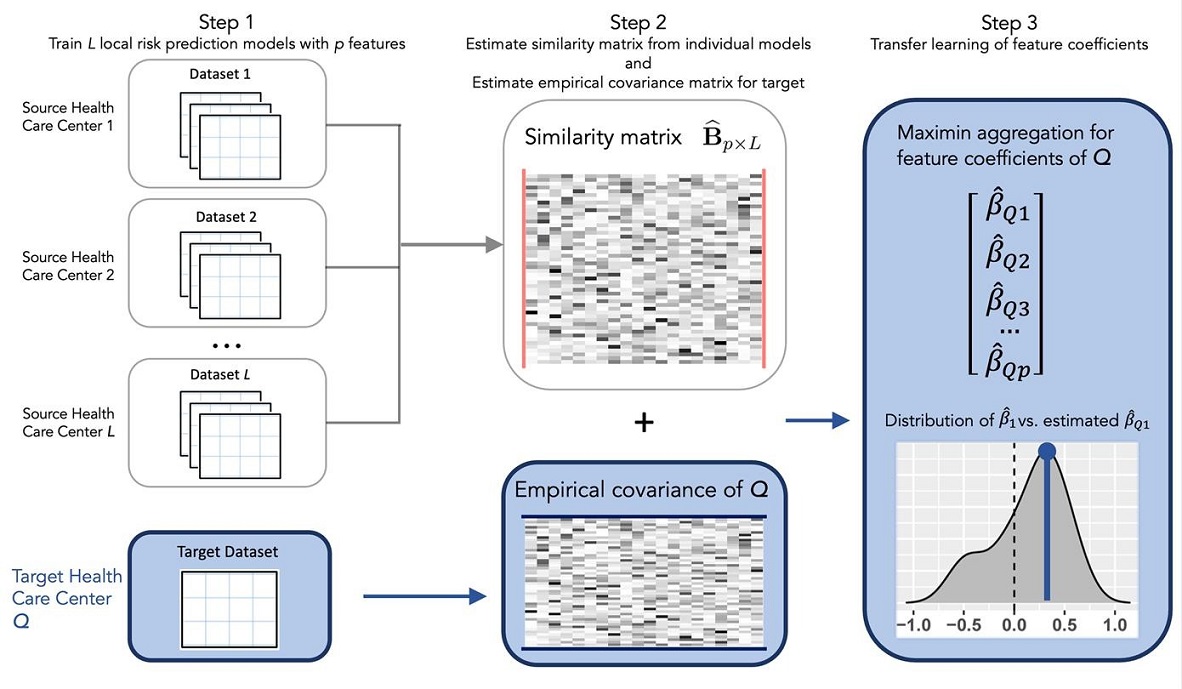
The training of ARRTLE contains three steps:

• Calculating the empirical variance covariance matrix at the target population, and the fitted model parameters at L healthcare centers.

• Compute a similarity matrix among the L models based on their coefficients. This matrix helps to understand how similar the source populations when applied to the target population.

• Apply a maximin aggregation process, which involves solving a penalized optimization problem to determine the optimal weights for each of the L models.

The ARRTLE algorithm essentially is to find a linear combination of the Cox regression vectors from each source model that best predicts the time-to-event outcome for the target population. The optimal weight learn from Maximin aggregation geometrically is the point that has the smallest distance to the origin and lies on the convex combination of the regression vectors.

The only requirement for training is the empirical covariance matrix and the fitted model parameters, free of any patient-level data.

To read more about ARRTLE, you can view or paper published at JBI.

You can also view our R package on github for additional information on formatting and creating the required inputs for the web app.

Quick Start Guide

Step 0 (optional): Train L Cox Models

Begin by training L Cox models, each utilizing the same set of p features. This step is optional if you’ve already fitted your models. For fitting a Cox model in R, the coxph() function from the survival package is recommended. Consider adding penalization for high-dimensional models to enhance stability and performance.

Step 1: Assemble Your Inputs

• Gather Estimated Coefficients: Compile the estimated coefficients from the models trained in the preparatory step into a matrix of dimensions p by L, where each column represents the p coefficients from one of the models.

• Empirical Variance-Covariance Matrix: Include the p by p empirical variance-covariance matrix for your target population’s features. If your target population spans multiple sites, provide a separate matrix for each.

Step 2: Determine the Need for Validation

If you have access to a validation dataset, opt for validation by uploading the dataset. Ensure the first column indicates the time to the event, followed by a censoring indicator column (1 for event occurrence, 0 for censoring). The subsequent columns should contain the p features used in the model, aligned in the same order as the coefficients in Step 1.

Step 3: Choose Your Learning Setting

Your choice of learning setting depends on the variance-covariance matrices provided:

• Transfer Learning: Select this option if you’ve uploaded a single variance-covariance matrix. It’s ideal for focusing on adapting insights from one source to the target population.

• Federated Learning: Choose federated learning if you’ve provided multiple variance-covariance matrices.

Step 4: Visualize and Download Your Results:

After completing the initial steps, it’s time to explore the insights generated by ARRTLE:

• Visual Insights: Dive into the “Heatmap”, “Density Plots”, and “Valid_Barplots” tabs for a comprehensive visual analysis. These tools offer intuitive visualizations to help you understand the similarities and distributions of the input and output models.

• Downloadable Results: visit the “Table” section to access and download the exact parameters of your fitted model.

Data format for this app

Transfer learning setting (only one target)

• Local estimators: a p-by-L matrix where each column stands for the coefficient estimation from a local site, stored as an .rds file.
• Target covariance matrix: a p-by-p covariance matrix extracted from the target site, stored as an .rds file.
• (Optional) Target validation data: a three-element R list, stored as an .rds file:
  • x: a numeric vector of length N, indicating the event time for each subject in the validation data.
  • delta: a logical vector of length N, indicating the event status (1: death; 0: censored).
  • z: an N-by-p matrix including covariates for each subject.

Federated learning setting (each local site can be the target)

• Local estimators: a p-by-L matrix where each column stands for the coefficient estimation from a local site, stored as an .rds file.
• Target covariance matrices: an L-element list where each element contains a p-by-p covariance matrix extracted from one local site, stored as an .rds file.
• (Optional) Target validation data: a three-element R list:
  • x: an L-element list where each element contains a numeric vector of length N, indicating the event time for each subject in the validation data from a local site.
  • delta: an L-element list where each element contains a logical vector of length N, indicating the event status (1: death; 0: censored) for subjects from a local site.
  • z: an L-element list where each element contains an N-by-p matrix including covariates for each subject from a local site.